While it’s fine to work with one of those many datasets which are publicly available, its a whole different task to come up with your own classification task and data. So for this project, I came up with my very own image classification problem, because I wanted to finally work with some real world data (not that all of the other publicly available datasets are not real, with real I mean that I wanted to actually choose something that was more hands on for me).
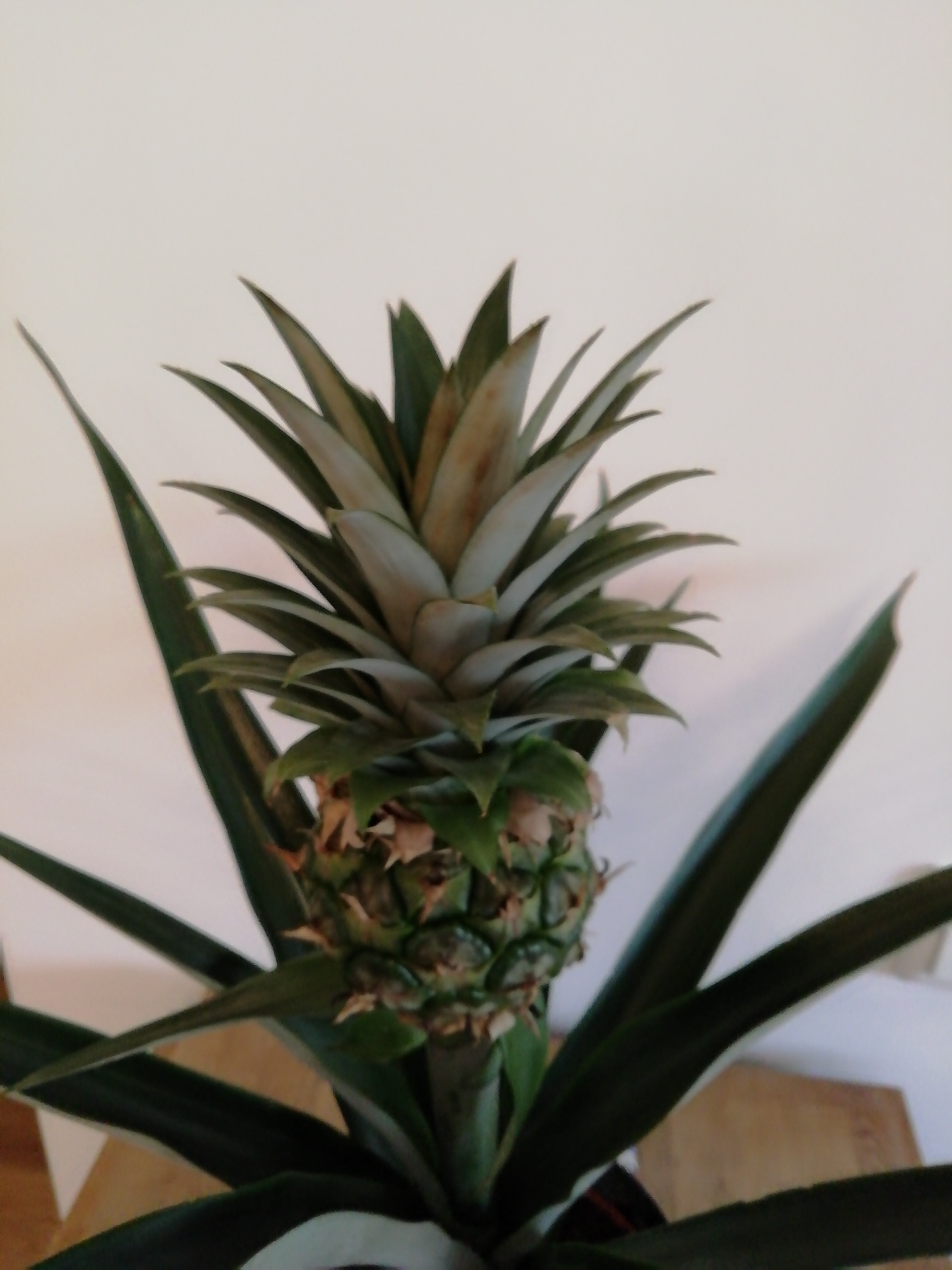
Having dealt with some very basic image classification in another project, the MNIST Digit Recognition example, I felt like I had to take it up a notch and apply the same principles to something else. On my quest to find something suitable, I came across the small Pineapple plant in my flat. So I thought, why not take multiple images from the Pineapple plant and also take multiple images from another plant (Yukka) and try to teach an algorithm to differentiate between those based on pixel data only. So I began to take some random pictures with my smartphone from all sorts of angles from both the Ananas and Yukka plant.
Ananas and Yukka image from the train set


The first issue I encountered: I takes soo long to take pictures. At least for me I guess. However, I thought there has to be a much more efficient way on how to generate enough images from all possible angles for this classification task. Well, there certainly is. I thought, why not record a video from both plants from all angles and then write a small program in Python that saves all frames from each video. I knew there would probably be some loss in quality for each image, but that was fine for me.
Code that I used to extract frames from a video
import cv2
print(cv2.__version__)

vidcap = cv2.VideoCapture('/Users/niklaskuehn/VID_20191011_163703.mp4')
success,image = vidcap.read()
count = 0
success = True
while success:
  cv2.imwrite(f"frame#{count}.jpg", image)
  success,image = vidcap.read()
  print(f"Read a new frame: {success}")
  count += 1
Depending on how many frames per second your phone camera is able to record videos, the more frames or images you get per second of video material. In my case, my Huawei smartphone was recording at 30fps, which resulted in about 1.800 images per minute of video recording. That really helped me to get some more training data in. So let’s get into actually coding some stuff.
Step 1 Importing Libraries and Images
import numpy as np
import os
import cv2
import random
import pickle

DATADIR = "/Users/niklaskuehn/Desktop/Python and Machine Learning/Own Img Datasets/Ananas Yukka Test/Train"
CATEGORIES = ["Ananas", "Yukka"]

IMG_SIZE = 150
training_data = []

def create_training_data(): ### Function that appends each image in the directory to the training_data List
    for category in CATEGORIES:
        path = os.path.join(DATADIR, category)  # path to cats or dogs dir
        class_num = CATEGORIES.index(category)
        for img in os.listdir(path):
            try:
                img_array = cv2.imread(os.path.join(path, img), cv2.IMREAD_GRAYSCALE)
                new_array = cv2.resize(img_array, (IMG_SIZE, IMG_SIZE))
                training_data.append([new_array, class_num])
            except Exception as e:
                pass

create_training_data()
Step 2 Shuffling Training Data and append Features and Labels
random.shuffle(training_data) ### Very important to shuffle the data at before training

X = []
y = []

for features, labels in training_data:
    X.append(features)
    y.append(labels)

X = np.array(X).reshape(-1, IMG_SIZE, IMG_SIZE, 1)

pickle_out = open("X.pickle", "wb") ### Saving the dataset using pickle, so loading the data is actually faster and we do not always need to form the dataset again
									### If you are working on a Jupyter Notebook you don't really need to save using pickle, but when running on console or in editor
  									### highly suggested to save the data and run the actual algorithm in a separate Python file
pickle.dump(X, pickle_out)
pickle_out.close()

pickle_out = open("y.pickle", "wb")
pickle.dump(y, pickle_out)
pickle_out.close()
Step 3 Creating the Model (in separate Python File)
import pickle
import time
from tensorflow.python.keras.models import Sequential
from tensorflow.python.keras.layers import Dense, Dropout, Activation, Flatten, Conv2D, MaxPooling2D
from tensorflow.python.keras.callbacks import TensorBoard


X = pickle.load(open("X.pickle", "rb"))
y = pickle.load(open("y.pickle", "rb"))

X = X/255.0

### If you want to test different parameters, you can simply add some more dense/convolutional layers in here if you would like
### Also you could change the layer sizes to whatever you want. For my algorithm I found that 0 Dense layers, 3 Convolutional layers
### and a layer size of 64 resulted in the highest accuracy. However when using a different dataset, other parameters might lead to
### more accurate results. Changing the parameters would look like:

### dense_layers = [0, 1, 2]
### layer_sizes = [32, 64, 128]
### conv_layers = [1, 2, 3]

### Results of the different Models can then be viewed in Tensorboard

dense_layers = [0]
layer_sizes = [64]
conv_layers = [3]

for dense_layer in dense_layers:
    for layer_size in layer_sizes:
        for conv_layer in conv_layers:
            NAME = "{}-conv-{}-nodes-{}-dense-{}".format(conv_layer, layer_size, dense_layer, int(time.time()))
            print(NAME)

            model = Sequential()

            model.add(Conv2D(layer_size, (3, 3), input_shape=X.shape[1:]))
            model.add(Activation('relu'))
            model.add(MaxPooling2D(pool_size=(2, 2)))

            for l in range(conv_layer-1):
                model.add(Conv2D(layer_size, (3, 3)))
                model.add(Activation('relu'))
                model.add(MaxPooling2D(pool_size=(2, 2)))

            model.add(Flatten())
            for _ in range(dense_layer):
                model.add(Dense(layer_size))
                model.add(Activation('relu'))

            model.add(Dense(1))
            model.add(Activation('sigmoid'))

            tensorboard = TensorBoard(log_dir="logs/{}".format(NAME))

            model.compile(loss="binary_crossentropy", optimizer="adam", metrics=["accuracy"])

            model.fit(X, y, batch_size=16, epochs=10, validation_split=0.15, callbacks=[tensorboard])

model.save('64x3-CNN.model') ### Best model in my case
Step 4 Actually working with the Data
If you wanted to actually work with your data you could simply use the following code to test the model on some new, unseen data. You could also take the model for example to create an App that would take pictures using the camera and then automatically classify the image.
import cv2
import tensorflow as tf

CATEGORIES = ["Ananas", "Yukka"]

def prepare(filepath):
    IMG_SIZE = 150
    img_array = cv2.imread(filepath, cv2.IMREAD_GRAYSCALE)
    new_array = cv2.resize(img_array, (IMG_SIZE, IMG_SIZE))
    return new_array.reshape(-1, IMG_SIZE, IMG_SIZE, 1)

model = tf.keras.models.load_model("64x3-CNN.model")

prediction = model.predict([prepare("Ananas 1 Test.jpg")])
print(CATEGORIES[int(prediction[0][0])])